As part of a work placement with Linguistic DNA, University of Sheffield MA student Winnie Smith has been examining the metadata that accompanies the Text Creation Partnership transcriptions of Early English Books Online (EEBO-TCP). Released as a CSV file (here), it combines the various codes that are used to identify different formats of EEBO (and related products). It also includes basic information like author, title, and date of publication. The focus of Winnie’s work described here are the “terms” or “subject headings”, which represent earlier attempts at cataloguing the items in the collection. What can these tell us about what’s in our main dataset?
Winnie writes:
One of the main reasons I’d applied to do a placement with LDNA was the opportunity to work with historical text, so I was very happy be given the chance to analyse EEBO-TCP metadata. Time disappears browsing EEBO (I never knew an agnus dei could be a little wax figurine as well as a mass movement), but I soon realised that analysing it in any depth is a pretty warts and all experience.
The initial target was to select a narrow date range, say 1610-1612, and try to identify broad genre and / or format categories for EEBO documents in that period (e.g. sermons, broadsides, or biographical works). The data sent back from this probe would then help LDNA in its mission to explore the “universe of printed discourse”.
However, getting the data turned out to be more complicated than it first appeared. I decided early that trying to determine semantic categories manually was both unsystematic and impractical. For 1610 alone, for example, there were 49 overtly Christian terms. How should they be grouped together? What about the classifications that might not apply to that year, but arise in other years?
In addition, the fact that the category labels in the metadata originated in the English Short Title Catalogue (ESTC), and had been provided in different ways by different people, meant that there were considerable differences in how texts were catalogued, leading to uncertainty about how they should be classified. There is also the potential for category clashes between modern labels and early modern concepts, for example of non-Christian religions. For example, did thematic entries which mentioned “Jews” refer to Jewish religious texts, learned works, or anti-Semitic material which within an Early Modern frame might claim to be religious and / or scholarly?
Terms from below
I therefore switched to looking for semantic clusters which might emerge directly from the terms. This approach had definite benefits. By manually splitting and sorting the single “Terms” column (using semicolons as the delimiter), I was able to see categories I would have missed if I had continued to rely on manual semantic classification, e.g. “broadsides”:

Figure 1: “Broadsides” emerging as a category in alphabetically sorted TCP metadata.
I also noticed that there were different kinds of categories present in the terms: far from all groupings being topic-based (e.g. repentance), there were several kinds of classification—in the case of broadsides, by printed format.
However, alphabetical manual sorting was time-consuming, and not guaranteed to unite similar content. For example, the entry
Conspiracies — Sermons — Early works to 1800. (A07558)
appeared separately from
Sermons, English — 17th century (A14860).
I decided to try and address that problem by further splitting, though this was complicated by different cataloguers punctuating in different ways. This made it difficult to split off information that wanted separating without separating information that didn’t. For example, all records use a double hyphen (–) to separate off separate units within a single classification. However, in the following record, a double hyphen appears within a single unit (James I) as well as between separate units, e.g. James I | King of England:
James — I, — King of England, 1566-1625. — Triplici nodo, triplex cuneus — Early works to 1800 (A20944)
After some pre-processing in Excel to try and make the punctuation and contents of the terms column more consistent (removing full stops; replacing double hyphens in front of regnal numbers; filtering out blanks or replacing them with dummy text), I loaded it into Rstudio, full of analytical idealism.
This was where the fun began.
The metadata contains widely differing numbers of term entries for different records. I had gravely underestimated the difficulties this would pose in R, which requires rows and columns to be of equal length. The issue was only compounded by the fact that the required number of new term columns (n) was also unknown. I eventually got round this by finding n first (56, as it turns out), then making all rows have n columns. This isn’t a particularly elegant coding solution, particularly because it uses multiple for-loops (which I know R frowns on) and these were slow for a dataset of over 53,000 rows. There are also issues about essentially counting a construct, X, as a proxy for term entries, where
X = something between one semicolon and another.
Observations
Caveats aside, this procedure enabled some interesting observations. The frequency of individual terms, for example, has a very long tail: 16997 items (63% of the total), occur only once. Sorting the terms alphabetically shows that there is still a great deal of noise, at least at the lower end:

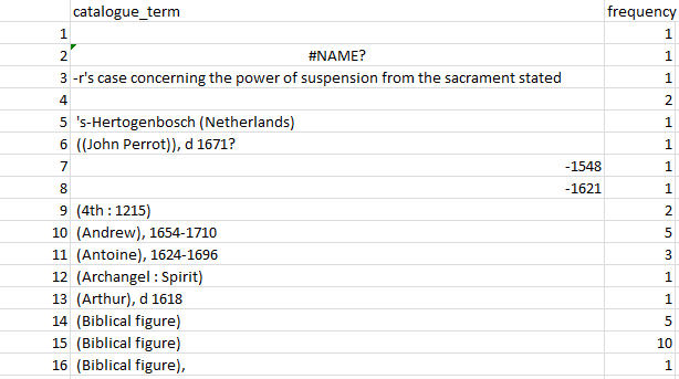
Figure 2: A snapshot of alphabetically sorted individual “terms” and their frequencies.
This snapshot from the output table (Figure 2) shows that some rows, e.g. 3, have been split incorrectly, despite pre-processing to try and deal with different numbers of hyphens. Other potentially tricky cases are correct (e.g. row 5). For some rows (e.g. 14–15) hidden characters clearly affected the result, and it might be worth adding extra processing steps. (I didn’t, for example, remove brackets or capitalisation.)
However, the process worked and was worth it. Even accepting that treating X as a distinct unit is an approximation for catalogue terms, and that the results are imperfect, being able to see the full number and range of cataloguing terms used in the EEBO-TCP metadata (294 378 total term quasi-tokens representing 26 858 unique quasi-types) frees them up for further independent manipulation.

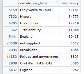
Figure 3: Top 10 cataloguing terms in EEBO-TCP metadata (by frequency).
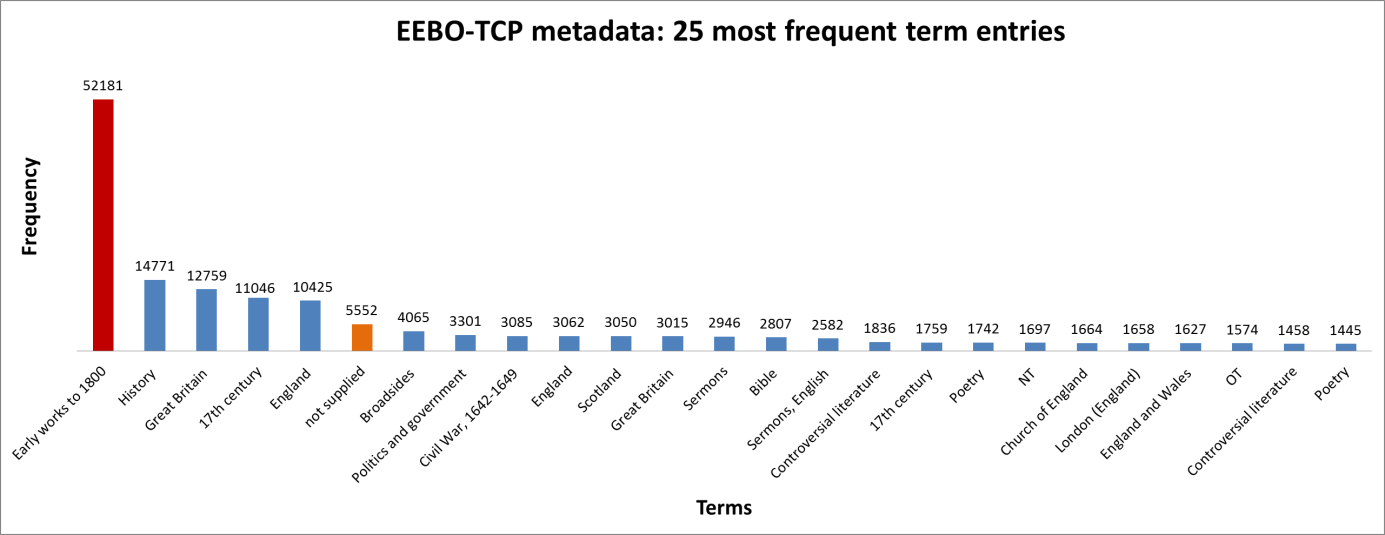
It was also instructive to see which expressions (with X ≈ terms) were most frequent in the dataset. Figure 3 (right) shows the top 10, while Figure 4 (below) visualises the relative distribution of the top 25.

Figure 4: The 25 most frequent cataloguing terms in EEBO-TCP metadata.
As the bar chart shows, by far the most frequent catalogue term is wholly uninformative: all works in EEBO-TCP are pre-1800, so “early literature to …” only confirms the selection criteria which apply to the dataset.
Perhaps more interesting is that the 6th most frequent item is “not supplied”; this shows how many records lack any kind of cataloguing information: “not supplied” was a dummy entry I inserted to remove blanks in pre-processing.
EDIT (7/7/17): We now realise the 2473 works from ECCO-TCP were inadvertently included in the term processing, inflating the reported blank count (“not supplied”). The true count for EEBO-TCP is 3102 items without terms, or ~6% of the total. Only 23 ECCO items have subject headings, with 2 containing the phrase “Early works to 1800”.
Keen-eyed readers may also have spotted “England” twice in the top terms, an artefact of stray spaces (following term-splitting). Removing this irregularity, we find 20,074 unique term-units; extracting commas and parentheses leaves 19864 distinct units—the various biblical figures of Figure 2 (lines 14-16) now represented by one common “biblicalfigure”.
This [nevertheless] shows that messiness extends to the upper as well as lower frequency limits of the dataset, though perhaps in a different sense: at the higher extreme, the issue appears to be less one of dealing with potentially large numbers of small inaccuracies, and more one of high-frequency results which are not all equally useful for semantic analysis.
However, one of the things I have learned on this placement is that no result is unwelcome. Unsurprisingly, EEBO-TCP was never designed for the type of digital text analysis LDNA conducts, meaning LDNA-type processes aren’t always intuitive to apply, but this does not detract from the benefits of working with EEBO, even (especially if) the results remind you to proceed with caution.
On a more personal level, the EEBO-TCP metadata is not the easiest thing to handle as a beginner (I did vainly wish it better, quite a lot), but extremely valuable for precisely that reason. Although I didn’t get much further than writing (cracking) the code to extract individual terms from the master dataset and beginning some summary statistics, I learned a vast amount about being pragmatic and patient with your data (and your programming environment), documenting your working, and the pain of struggling to make sense of messy, non-textbook data is in fact an inevitable part of the process I most enjoy: working with historical text which was never written for a machine to breeze through.
As I finish my placement, I hope my results will allow LDNA to continue analysing EEBO-TCP in more depth, and I’m looking forward to continuing the different kinds of pleasure that come from text analysis (from wonder to perseverance) into a PhD.
Note: For those who might wish to replicate Winnie’s work (noting the disclaimer about inelegant code), here is closer documentation of that process:
I used the following procedure:
a) find n
1) looping over each row of the dataset and calculating the number of term entries for each record
2) adding each result to a vector of term lengths (see code extract 1, below)
3) finding the largest number in this vector (see code extract 2, below)
b) create equal numbers of split terms for each record
4) looping back over the dataset, splitting each row, and making up any difference between the number of terms for that record and the maximum number of terms by adding missing values (NAs) so that each row was of equal length.
c) combine all the newly created term columns into a single column, removing the missing values.

Code extract 1 (above). Code extract 2 (below).

 It is Writing as Resistance.



 ANNALISA TOCCARA is a Marketer & PR professional, Community Activist & Creative Director. Based in Sheffield and founder of the social enterprise Our Mel, Annalisa launched Sheffield’s first Black History Month Festival; MelaninFest® in October 2017, which saw a total of 43 events spread across the month in collaboration with over 40 partners and also launched a sister festival in London. Since then, Annalisa has hosted a number of community events celebrating Black excellence, Black talent and Womanhood. Through her work with Our Mel and previous social justice endeavours, she has developed a passion for arts and culture having seen first-hand how creative mediums can help shape and create social cohesion within our community. Annalisa also has a BA (Hons) in Biblical Study and Applied Theology with a Diploma in Leadership and is currently studying for her Chartered Marketer status. She is also the Vice-Chair of the BAMER Hub – Sheffield’s Equality Hub Network.


