Tag Archives: proximity data

Dr Kris Heylen at the Humanities Research Institute, Sheffield

Learning with Leuven: Kris Heylen’s visit to the HRI

In 2016, Dr Kris Heylen (KU Leuven) spent a week in Sheffield as a HRI Visiting Fellow, demonstrating techniques for studying change in “lexical concepts” and encouraging the Linguistic DNA team to articulate the distinctive features of the “discursive concept”.


Earlier this month, the Linguistic DNA project hosted Dr Kris Heylen of KU Leuven as a visiting fellow (funded by the HRI Visiting European Fellow scheme). Kris is a member of the Quantitative Lexicology and Variational Linguistics (QLVL) research group at KU Leuven, which has conducted unique research into the significance of how words cooccur across different ‘windows’ of text (reported by Seth in an earlier blogpost). Within his role, Kris has had a particular focus on the value of visualisation as a means to explore cooccurrence data and it was this expertise from which the Linguistic DNA project wished to learn.

Kris and his colleagues have worked extensively on how concepts are expressed in language, with case studies in both Dutch and English, drawing on data from the 1990s and 2000s. This approach is broadly sympathetic to our work in Linguistic DNA, though we take an interest in a higher level of conceptual manifestation (“discursive concepts”), whereas the Leuven team are interested in so-called “lexical concepts”.

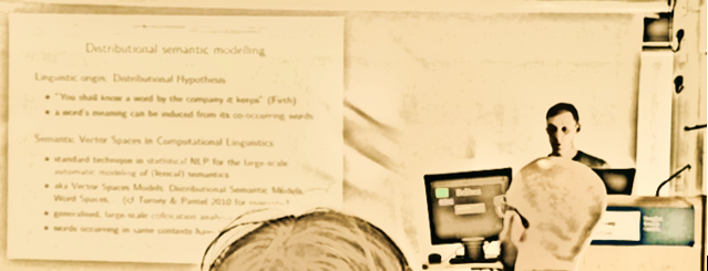
In an open lecture on Tracking Conceptual Change, Kris gave two examples of how the Leuven techniques (under the umbrella of “distributional semantics”) can be applied to show variation in language use, according to context (e.g. types of newspaper) and over time. A first case study explored the notion of a ‘person with an immigration background’ looking at how this was expressed in high and low brow Dutch-language newspapers in the period from 1999 to 2005. The investigation began with the word allochtoon, and identified (through vector analysis) migrant as the nearest synonym in use. Querying the newspaper data across time exposed the seasonality of media discourse about immigration (high in spring and autumn, low during parliamentary breaks or holidays). It was also possible to document a decrease in ‘market share’ of allochtoon compared with migrant, and—using hierarchical cluster analysis—to show how each term was distributed across different areas of discourse (comparing discussion of legal and labour-market issues, for example). A second comparison examined adjectives of ‘positive evaluation’, using the Corpus of Historical American English (COHA, 1860-present). Organising each year’s data as a scatter plot in semantic space, the path of an adjective could be traced in relation to others—moving closer to or apart from similar words. The path of terrific from ‘frightening’ to ‘great’ provided a vivid example of change through the 1950s and 1960s.

During his visit, Kris explored some of the first outputs from the Linguistic DNA processor, material printed in the British Isles (or in English) in two years, 1649 and 1699, transcribed for the Text Creation Partnership, and further processed with the MorphAdorner tool developed by Martin Mueller and Philip Burns at NorthWestern. Having run this through additional processes developed at Leuven, Kris led a workshop for Sheffield postgraduate and early career researchers and members of the LDNA team in which we learned different techniques for visualising the distribution of heretics and schismatics in the seventeenth-century.

The lecture audience and workshop participants were drawn from fields including English Literature, History, Computer Science, East Asian Studies, and the School of Languages and Cultures. Prompted partly by the distribution of the Linguistic DNA team (located in Sussex and Glasgow as well as Sheffield), both lecture and workshop were livestreamed over the internet, extending our audiences to Birmingham, Bradford, and Cambridge. We’re exceedingly grateful for the technical support that made this possible.

Time was also set aside to discuss the potential for future collaboration with Kris and others at Leuven, including participation of the QLVL team in LDNA’s next methodological workshop (University of Sussex, September 2016) and other opportunities to build on our complementary fields of expertise.


Proximity Data II: Co-occurrence and distance measurements

In a previous post, we addressed proximity data by defining proximity, term, and co-occurrence. In this post, we weigh specific options for measuring co-occurrence. In particular, we look at an array of distance measurements or windows for co-occurrence. In the Linguistic DNA project, we will be experimenting with many of the options and approaches below. Options for measuring co-occurrence and distance include the following.


Text Co-occurrence

Measures of text co-occurrence are generally used to measure similarity between texts. Put simply, a word frequency list is generated for each text, and frequency lists can then be compared across texts. Texts with similar frequency lists are considered to contain similar content.

The technical developers for Linguistic DNA have already begun compiling some frequency data using the programming language R.  The text mining package that accompanies R includes a measure of text co-occurrence, which can be analysed statistically within R (a matter for a separate blog post). In general, when investigating text co-occurrence, word order is ignored, as are grammatical relationships, including clause and sentence boundaries.

But boundaries can be significant.


Paragraph Co-occurrence

Rather than measuring co-occurrence in a complete text, it is also possible to measure co-occurrence paragraph by paragraph, using a similar approach. In addition to indicating paragraph topic, this approach can also be used for lexical semantics. In Landauer and Dumais’s (1997) approach, two terms that tend to co-occur within a single paragraph are likely to represent similar conceptual fields and even to be near-synonyms. They found this approach to be successful in machine learning of synonyms.

However, such an approach would likely be problematic for Linguistic DNA, as the coding applied to EEBO was not much occupied by paragraphing. Moreover, the deployment and purpose of paragraphs has evolved so that their value as a semantic determiner may not be the same in the 1500s as for modern texts.


Another mechanism is to impose boundaries by counting words to left and right. A variety of ‘windows’, or distances to the left and right, are possible. We discuss them below from the widest window to the narrowest window.


+/- 10 words

Burgess and Lund (1997) describe using a window of +/-10 words in their Hyperspace Analogue to Language. That is, they count all words within the range of 10 words to the left and right of each node. A frequency list is made for the window around each node, and frequency lists can then be compared for different nodes. Burgess and Lund (ibid.) claim psycholinguistic validity for this 10-word window, arguing that this represents the number of words held in working memory by a human listener/reader. They ignore word order and grammatical relations, including clause and sentence boundaries.

A word list with this window could be created with weightings that reflect distance from the node: the term that is 10 words to the left or right of the node can be weighted less than the term immediately to the left or right of the node. Such weighting would presume that words occurring in closer proximity are more likely to be semantically related than words that occur further apart.


Up to +/- 5 words

A window of up to +/- 5 words is quite common, and many researchers have used windows of +/-5 words, +/-3 words, or +/-1 word. That is, of course, not to say that this is the best choice in any or all circumstances. Indeed, it is perhaps computationally heuristic – a count and a unit (the word) that most computing technology can cope with.


2 words to the left

Many part of speech taggers (including MorphAdorner’s) rely on trigrams consisting of a node word and two words to the left (cf. Manning and Schuetze 2001, Chapter 10). This is considered a reliable standard in the field for identifying part of speech. Additional words to the left or right seem to produce diminishing returns in reliably tagging parts of speech. Word order is crucial. Experimentation with this window for semantic studies is limited and there is no reason to presume that this window would be useful for semantic information.


+/- n Content Words

A common step in analysing proximity data is to catalogue all co-occurrences within a window and then remove stop words such as grammatical/function words such as determiners (e.g. a, an, the) and prepositions (e.g. of, in, from). Depending on the research question, researchers may be less interested in grammatical/function words such as determiners and prepositions and more interested in the content/lexical words that co-occur with a node.

A variation on this approach is to strip such stop words from the corpus data first, and then to catalogue the n (e.g. 5) content/lexical words to the right and left of the node. As far as we’re aware, this approach has not been employed in published studies.


Assessing the Proximity Windows

Which window is best? That depends in part on your research questions. Larger windows seem to be better for some things, and smaller windows seem to be better for some things – and incorporating grammatical relationships into the window may be best of all for some questions. According to Sahlgren (2006; cf. Heylen et al. 2015) and Turney and Pantel (2010), extending proximity measurement to larger windows such as document co-occurrence (disregarding word order) is most useful for modelling syntagmatic and associative relations (or relational similarity) such as that between ‘doctor’ and ‘hospital’ or ‘car’ and ‘drive’. Proximity measurements using a narrow window can best indicate paradigmatic relations (or attributional similarity) like that between near-synonyms ‘hospital’ and ‘clinic’. Measuring grammatical relationships improves semantic findings for proximity measurements using narrow windows. Indeed, incorporating syntactic data can be extremely valuable for lexical semantic investigations, but, alas, it is not always possible.


Moving Forward

Linguistic DNA is beginning to design an automated method to draw proximity data from EEBO and ECCO. We call this automated method a semantic parser, or, with varying degrees of irony, a magic parsing box. This parser is being built one step at a time, tested on a dataset, and then assessed and developed further. At this stage, therefore, we are working with a proto-parser.

The first step for the proto-parser is to index the simplest lexical co-occurrences at a window of +1, -1, and the aggregate +/-1, for every word (type) in a small, random sub-sample of EEBO. Such a small window may or may not be terribly informative for lexical semantics – we’ll see – but it is a practical step in the prototyping process. From there, we will build up to measure more extensive co-occurrence data like that described above, and to incorporate the types of lexical relationships described in the previous post. We plan to build up in independent steps, assessing and evaluating the results of each step, what we can learn from it and what we can’t. We’ll document that process here on the blog. Ultimately, we aim to aggregate and weight these proximity measures as part of the broader goal of profiling each word in EEBO and ECCO.


Works Cited

Burgess, Curt and Kevin Lund. Modelling Parsing Constraints with High-dimensional Context Space. Language and Cognitive Processes 12 (2/3), 177–210.

Heylen, K., T. Wielfaert, D. Speelman, D. Geeraerts. 2015. Monitoring Polysemy: Word Space Models as a Tool for Large-Scale Lexical Semantic Analysis. Lingua 157, 153-72.

Landauer, Thomas K. and Susan T. Dumais. 1997. A Solution to Plato’s Problem: The Latent Semantic Analysis Theory of Acquisition, Induction, and Representation of Knowledge. Psychological Review 104 (2), 211-40.

Manning, Christopher and Hinrich Schuetze. 2001. Foundations of statistical natural language processing. Boston: MIT Press.

Sahlgren, M. 2006. M. The Word-Space Model: Using Distributional Analysis to Represent Syntagmatic and Paradigmatic Relations Between Words in High-dimensional Vector Spaces. (Ph.D. dissertation), Department of Linguistics, Stockholm University.

Turney, Peter D. and Patrick Pantel. 2010. From Frequency to Meaning: Vector Space Models of Semantics. Journal of Artificial Intelligence Research 37, 141-188.

Proximity Data

Background

The Linguistic DNA project will be interrogating cleaned-up EEBO and ECCO data in various ways, to get at its lexical semantic and conceptual content. But how do we get semantic and conceptual information from textual data? Sticking with  the original project proposal, we begin with an analysis of ‘proximity data’. What is proximity data, what does it tell us, and how can we measure it?

What is proximity?

Proximity relates to co-occurrence between terms in language. So, what is a term and what does it mean to co-occur?

A term may be:

  • a single word, a pair of words (or bigram), or a string of three or more words in order (an n-gram);
  • a grammatical construction whose ‘slots’ can be filled with appropriate words (e.g. ‘NOUN of NOUN’, ‘ADJECTIVE as NOUN’, or even ‘VERB MODIFIER DIRECT OBJECT’);
  • a phrase with lexical wild cards such as ‘very ___ ideas’.

Co-occurrence can then be defined as the presence of two or more terms within a given set of data, or in a given relationship. For example, we might be interested in the co-occurrence of two single words like Lord and law: In which texts do those terms co-occur? How close is one to the other? Or, we might be interested in the co-occurrence of a single word with a grammatical pattern: In which texts is see followed by a subordinate clause?

How do we investigate proximity?

We can ask a few different things about the distance between terms that co-occur. For example, we can inquire: ‘What terms occur within a given distance of term a (e.g. Lord)?’ Or, we can ask: ‘How far is term a (e.g. Lord) from term b (e.g. law)?’ Put differently, we can measure co-occurrence by selecting a starting point term (a node) and a distance from that starting point, and seeing what terms occur within that distance. Alternatively, we can select multiple nodes as starting points and measure the distance between them in use. We can also combine these two methods: we can first ask what words occur within a given distance of term a, and then take pairs of words from the resulting list and ask just how closely they occur to each other.

Finally, we can ask: ‘What occurs in a given relationship to term a?’ These questions can be syntactic: ‘What are the Direct Objects and Subjects of term a (e.g. see)?’ or related to Parts Of Speech (POS) ‘What noun occurs most frequently after term a (e.g. see)?’ We can also hypothetically ask about semantic relationships: ‘What is the Agent or Patient, Instrument or Theme related to term a?’ A syntactic approach is employed by the commercially-developed Sketch Engine software, and also generally, in various ways, in the Behavioural Profiling technique used by Stefan Gries (2012), in the collostructional approach used by Anatol Stefanowitsch and Gries (2008) and by Martin Hilpert (2012). This approach requires either satisfactory automated syntactic parsing or manual syntactic parsing—both of which seem to be impossible with EEBO because of the scale and variation documented previously. A POS approach is more viable with EEBO, but still difficult.

An alternative to syntactic and POS approaches is pair-pattern matrices: rather than investigating co-occurrence within grammatical relationships, we can investigate co-occurrence within given lexical structures such as ‘a cut(s) b’, ‘a work(s) with b’, etc. This has been explored in machine learning and artificial intelligence research (Turney and Pantel 2010).

What does proximity data tell us?

Proximity data represents a relatively data-driven approach to corpus semantics (and to semantic analysis in Natural Language Processing [NLP], artificial intelligence, data science, and other fields). In linguistics, the use of proximity data in this way is based upon the idea that words occurring together or in similar contexts are likely to share a similar meaning or occupy a similar conceptual field. This is known as a contextual theory of meaning, and in its early stages the theory was developed in particular by J. R. Firth, Michael Halliday, and John Sinclair (cf. Stubbs 1996; Oakey 2009). Sinclair pioneered the application of the theory in lexicography, with the Collins COBUILD Dictionary. That dictionary designed its entries around the most frequent collocational patterns for each dictionary headword, as evidenced by corpus data. In addition to lexicographical applications, proximity data are now used to study lexical semantics; to automatically identify Parts of Speech; to generate computer models of linguistic meaning in NLP and artificial intelligence studies; as well as to engineer text search tools, summarise texts, identify text topics, and even analyse writers’ ‘sentiment’ (cf. Manning and Schuetze 2001, Chapter 5).

But there is a crucial epistemological question that arises here. At its most basic level, co-occurrence data in corpora tell us directly about language use and usage. What is the link between corpus data showing lexical usage, on the one hand, and lexical semantics or conceptual fields, on the other? That is a question that will preoccupy Linguistic DNA as it evolves – and a question we will continue to address on the blog.

Works Cited

Gries, Stefan Th. 2012. Behavioral profiles: A fine-grained and quantitative approach in corpus-based lexical semantics. In Gary Libben, Gonia Jarema and Chris Westbury (eds), Methodological and analytic frontiers in lexical research. Amsterdam: John Benjamins Publishing Company. 57-80.

Hilpert, M. 2012. Diachronic collostructional analysis meets the noun phrase. In T. Nevalainen and E. C. Traugott (eds.), Oxford Handbook of the English Language. Oxford 2012. 233–44.

Manning, Christopher and Hinrich Schuetze. 2001. Foundations of statistical natural language processing. Boston: MIT Press.

Oakey, David. 2009. Fixed collocational patterns in isolexical and isotextual versions of a corpus. In Paul Baker (ed.), Contemporary corpus linguistics. London, Continuum. 140-58.

Stefanowitsch, Anatol & Stefan Th. Gries. 2008. Channel and constructional meaning: A collostructional case study.  In Kristiansen and Dirven (eds.), Cognitive Sociolinguistics: Language variation, cultural models, social systems, 129-152. Berlin: Mouton de Gruyter.

Stubbs, Michael. 1996. Text and corpus analysis. Oxford: Blackwell.

Turney, Peter D. and Patrick Pantel. 2010. From Frequency to Meaning:
Vector Space Models of Semantics. Journal of Artificial Intelligence Research 37, 141-188.